DL with TF

Deep learning with Tensorflow

Matthew Greenberg University of Calgary Deptment of Mathematics and Statistics

mgreenbe@ucalgary.ca mgreenbe.github.io/mruai2019-slides/

What is Tensorflow?

"An end-to-end open source machine learning platform."

tensorflow.org

Tensorflow's strengths

Versatility:

Model development, training, inference

Performance:

Implemented in C++
GPU acceleration

Usability:

Consume using a Python or C++ API
High level Keras API for deep learning

Ecosystem

Libraries, extension, tooling

Tensorflow lite for mobile/IOT

Tensorflow Extended for production deployments

Officially curated and community contributed models and datasets

Forums, blogs, Youtube channel, > 46000 Stackoverflow questions tagged "tensorflow", ...

Importing

We'll be using Tensorflow 2.0.

On Colab:


				%tensorflow_version 2.x

Import as usual:


				import tensorflow as tf

Check your version:


				print(tf.version.VERSION)


			2.0.0-rc2

Tensors

$n$-dimensional arrays of numbers.

Construct them using tf.constant.

a = tf.constant(3) # dtype=int32
b = tf.constant([[3., 1., 4.], [1., 5., 9.]])
print(a, b)
print(b.__class__)

tf.Tensor(3, shape=(), dtype=int32)
tf.Tensor([[3. 1. 4.]
	   [1. 5. 9.]], shape=(2, 3), dtype=float32)
<class 'tensorflow.python.framework.ops.EagerTensor'>

Convert tensors to numpy arrays

c = b.numpy()
print(c, c.__class__)

[[3. 1. 4.]
 [1. 5. 9.]] <class 'numpy.ndarray'>

and vice-versa.

d = tf.constant(c)
print(d == b)

tf.Tensor([[ True  True  True]
           [ True  True  True]], shape=(2, 3), dtype=bool)

Unlike Numpy arrays, tensors are immutable

b = tf.constant([3., 1., 4., 1., 5., 9.])
b[0] = 4

TypeError: 'tensorflow.python.framework.ops.EagerTensor' 
           object does not support item assignment

and can be backed by GPU memory.


with tf.device("/device:GPU:0"):
    a = tf.constant([3., 1., 4., 1., 5., 9.])
    print(a.device)


								/job:localhost/replica:0/task:0/device:GPU:0

Variables

Variables are mutable tensors.

Typically contain trainable quantities, e.g. weights.

Make variables by passing an initial value to the tf.Variable constructor:

b = tf.Variable([3., 1., 4., 1., 5., 9.])
b.assign_add(tf.ones_like(b))
print(b)

<tf.Variable 'Variable:0' shape=(6,) dtype=float32,
numpy=array([ 4.,  2.,  5.,  2.,  6., 10.], dtype=float32)>

A simple training loop

Let's do simple linear regression with Tensorflow.

Mock up some data:

a_true = tf.constant(-0.25) # intercept
b_true = tf.constant(0.5)   # slope
x = tf.random.uniform((96,))
e = tf.random.normal((96,), 0, 0.1)
y = a_true + b_true*x + e

We want to fit a line to the dataset (x, y).

Select initial values for our trainable parameters — the intercept a and the slope b:

a = tf.Variable(0.)
b = tf.Variable(tf.random.uniform(()))

Choose a learning rate.

lr = tf.constant(0.5)

Write a training loop to perform gradient descent.

for epoch in range(100):                      # training loop
    with tf.GradientTape() as t:
        loss = tf.reduce_mean((a + b*x - y)**2)         # (*)
        [dloss_da, dloss_db] = t.gradient(loss, [a, b])
        a.assign_sub(lr*dloss_da)        # "a -= lr*dloss_da"
        b.assign_sub(lr*dloss_db)

print(a.numpy(), b.numpy())    # a_true = -0.25, b_true = 0.5

-0.2548124 0.5260704

tf.GradientTape() is a context manager that records details of computation (*) needed to compute gradients. (Consider it an implemention detail.)

A stochastic (batched) variant

a_true = tf.constant(-0.25) # true intercept
b_true = tf.constant(0.5)   # true slope

x = tf.random.uniform((96,))
e = tf.random.normal((96,), 0, 0.1) # errors in y
y = a_true + b_true*x + e

dataset = tf.data.Dataset.from_tensor_slices((x, y))

Same as previously. Mock up a dataset (x, y) for the purpose of fitting a linear model.

tf.data contains functionality for building data pipelines.

The tf.data.Dataset class is optimized for large datasets.

a = tf.Variable(0.) # initial intercept
b = tf.Variable(tf.random.uniform(())) # initial slope
lr = tf.constant(0.25) # learning rate

for x, y in dataset.shuffle(96) \
                   .repeat(100) \
                   .batch(3):
    with tf.GradientTape() as t:
        loss = tf.reduce_mean((a + b*x - y)**2)
        [dloss_da, dloss_db] = t.gradient(loss, [a, b])
        a.assign_sub(lr*dloss_da) # "a -= lr*dloss_da"
        b.assign_sub(lr*dloss_db)

Choose initial values for trainable parameters. Select learning rate.

Loop through the dataset 100 times in 3 batches of 32 samples. Shuffle it before each iteration.

Same as previously. Compute loss for batch. Compute gradients. Update a and b.

Keras

Tensorflow's high level API for deep learning.

Powerful, modular, composable, extensible, user friendly, well documented.

Prefer it to Tensorflow's lower level API, where feasible.

Keras models

A Keras model describes data flow through layers.

Each layer of a model encodes the weights of its connections to preceding layers.

A dense layer has a unique weight for each of these connections.


				from tensorflow.keras import Model, Sequential
				from tensorflow.keras.layers import Dense, Input

A simple feedforward network


				model = Sequential([Input(2), Dense(3), Dense(3), Dense(1)])

Model summary


						  model.summary()


Model: "sequential"
_________________________________________________________________
Layer (type)                 Output Shape              Param #   
=================================================================
dense (Dense)                (None, 3)                 9         
_________________________________________________________________
dense_1 (Dense)              (None, 3)                 12        
_________________________________________________________________
dense_2 (Dense)              (None, 1)                 4         
=================================================================
Total params: 25
Trainable params: 25
Non-trainable params: 0
_________________________________________________________________

Layers

Layers are stored on the model.layers

[<tensorflow.python.keras.layers.core.Dense at 0x13f3a0f50>,
  <tensorflow.python.keras.layers.core.Dense at 0x13f3b5410>,
  <tensorflow.python.keras.layers.core.Dense at 0x13f3b5990>]

Easy to get input about a given layer:

L = model.layers[0]
  print(f"L.name = {layer.name}, L.units = {layer.units},
          L.input_shape = {L.input_shape},
          L.output_shape = {L.output_shape}")

L.name = dense, L.units = 3,
L.input_shape = (None, 2), L.output_shape = (None, 3)

Inference model.predict

Inference is the process of predicting y from x by propagating data forwards through the network.

tf.random.set_seed(666)
x = tf.random.uniform((4, 2))
y_pred = model.predict(x)


x = [[0.7861 0.4992]
     [0.2993 0.8064]
     [0.8418 0.4165]
     [0.0332 0.8668]],

y_pred = [[ 0.5011]
          [-1.06  ]
          [ 0.7761]
          [-1.695 ]]

Understanding inference

A unit computes a weighted sum of its input values.

layers[0].get_weights()

[array([[0.8815, -1.0451, -0.9774],
aaaaaaa [1.0588, -0.1274, 0.4328]], dtype=float32),
aarray([0., 0., 0.], dtype=float32)]

Weighted sums are computed by matrix multiplication:

weights = [layer.get_weights() for layer in layers]

y = x
for [w, b] in weights:
    y = y @ w + b

y = [[ 0.5011]
     [-1.06  ]
     [ 0.7761]
     [-1.695 ]]

Layers are callable:

z = x
for layer in layers:                               
    z = layer(z)

z = [[ 0.5011]
     [-1.06  ]
     [ 0.7761]
     [-1.695 ]]

y and z are both equal to y_pred = model.predict(x).

Wait a second...

[[w1, b1], [w2, b2], [w3, b3]] = weights

w = w1 @ w2 @ w3
b = b1 @ w2 @ w3 + b2 @ w3 + b3
y = x @ w + b

y = [[ 0.5011]
     [-1.06  ]
     [ 0.7761]
     [-1.695 ]]

The model is linear! (Did you notice?)

To go beyond linear models, we need nonlinear activation functions.

Activation functions

Given input $x$, the output of a typical dense layer is \[ y = h(xW + b), \] where $W$, $b$, and $h$ are its weight matrix, bias vector, and activation function, respectively.

import tensorflow.keras.activations

Name	Shorthand	Formula	Use
identity	linear	$h(x)=x$	output layer in regression problems
sigmoid	sigmoid	$h(x)=\dfrac{1}{1 + e^{-x}}$	output layer in two-class classification problems
softmax	softmax	$h_i(x)=\dfrac{e^{x_i}}{\sum_{j=1}^K e^{x_j}}$	output layer in $K$-class classification problems
rectified linear unit (ReLU)	relu	$h(x)=\max(x, 0)$	hidden layers of deep networks

You can add an activation to a layer using the activation keyword argument in its constructor.

model = Sequential([Input(2),
    Dense(10, activation="relu"),
    Dense(10, activation="relu"),
    Dense(1, activation="sigmoid")])

Alternatively, you can add an activation "layer".

model = Sequential([Input(2),
    Dense(10), Activation("relu"),
    Dense(10), Activation("relu"), 
    Dense(1), Activation("sigmoid")])

Losses and optimizers

Learning algorithm = Model + Loss + Optimizer

Loss functions

Training a neural network means minimizing an appropriate loss function.

Name	Shorthand	Use
Mean squared error	mse	regression problems, continuous response
Binary cross-entropy	binary_crossentropy	two-class classification problems
Categorical cross-entropy	categorical_crossentropy	$K$-class classification problems

import tensorflow.keras.losses

Optimizers

All variants of stochastic gradient descent (sgd).

They all have tuneable parameters, the most important being learning rate (lr).

from tensorflow.keras.optimizers import SGD

optimizer = SGD(lr=0.005) # default lr = 0.01

Compiling a model

We endow a model with a loss function and an optimizer by compiling it.

model.compile(loss="mse", optimizer="sgd")

model.compile(loss="binary_crossentropy",
              optimizer=SGD(lr=0.005))

A compiled model is ready for training.

Metrics

Metrics are measurements measure quality of fit.

Loss functions are metrics. Other metrics might also be of interest, though.

The main examples of auxilliary metrics are training accuracy and validation accuracy.

Specify the metrics you want trackded in the metrics kwarg of your model's compile method.

model.compile(loss="binary_crossentropy",
              optimizer="adam",
              metrics=["accuracy"])

Training a model

Train a model using its fit method.

You need to provide training data, (x, y).

You can specify the number of epochs to train (epochs), batch size (batch_size), a validation split or dataset (validation_data, validation_split), and a sequence of callbacks (callbacks) in their respective kwargs.

model.fit(x_train, y_train,
          epochs=20,
          batch_size=64,
          validation_split=0.2)

Learning planar regions

Let's train a neural network to determine whether a random point in the unit square lies in the outer blue region or the inner red region.

Generate a training set of 512 randomly chosen points from the unit square, labelled accordingly.

a = 1/np.sqrt(8)

x_train = np.random.uniform(
    size=(512, 2))
    
y_train = np.logical_and(
    np.abs(x_train[:,0] - 0.5) < a,
    np.abs(x_train[:,1] - 0.5) < a))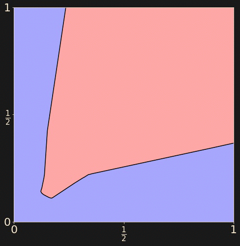

model = Sequential([Input(2),
Dense(10, activation="relu"),
Dense(10, activation="relu"),
Dense(1, activation="sigmoid")])

model.compile(
  loss="binary_crossentropy",
  optimizer="adam",
  metrics=["accuracy"])

model.fit(x_train, y_train, 
  epochs=500)

model.evaluate(x_test, y_test)

[0.100700, 0.9628906]

Saving models

The Model class has a save method.

This saves your model — both architecture the weights — in hdf5 format (.h5), optimized for storing multidimensional array data.

If you forget the .h5 extension, your model will be saved in protobuf (protocol buffer) format.

You'll run into protocol buffers if you work with non-Keras tensorflow models.

model.save("squares.h5")

Loading models

The tensorflow.keras.models module contains a load_model function:

from tensorflow.keras.models import load_model

model = load_model("square.h5")

Keras comes with many useful built-in models. They're located in tensorflow.keras.applications.

from tensorflow.keras.applications.vgg16 import VGG16

Colab notebooks

Pretrained networks

Transfer learning

Naive image denoising

Training loop for simple linear regression